Simple Introduction

This tutorial demonstrates the capability to perform ensembles of calculations in parallel using libEnsemble.

We recommend reading this brief Overview.

For this tutorial, our generator will produce uniform randomly sampled values, and our simulator will calculate the sine of each. By default we don’t need to write a new allocation function.

1. Getting started

libEnsemble is written entirely in Python. Let’s make sure the correct version is installed.

$ python --version
Python 3.8.0            # This should be >= 3.8

For this tutorial, you need NumPy and (optionally) Matplotlib to visualize your results. Install libEnsemble and these other libraries with

$ pip install libensemble
$ pip install matplotlib # Optional

If your system doesn’t allow you to perform these installations, try adding --user to the end of each command.

2. Generator

Let’s begin the coding portion of this tutorial by writing our generator function, or gen_f.

An available libEnsemble worker will call this generator function with the following parameters:

Input: A selection of the History array, passed to the generator function in case the user wants to generate new values based on simulation outputs. Since our generator produces random numbers, it’ll be ignored this time.

persis_info: Dictionary with worker-specific information. In our case, this dictionary contains NumPy Random Stream objects for generating random numbers.

gen_specs: Dictionary with user-defined static fields and parameters. Customizable parameters such as lower and upper bounds and batch sizes are placed within the gen_specs["user"] dictionary, while input/output and other fields that libEnsemble needs to operate the generator are placed outside user.

Later on, we’ll populate gen_specs and persis_info when we initialize libEnsemble.

For now, create a new Python file named generator.py. Write the following:

examples/tutorials/simple_sine/tutorial_gen.py

import numpy as np


def gen_random_sample(Input, persis_info, gen_specs):
    # Pull out user parameters
    user_specs = gen_specs["user"]

    # Get lower and upper bounds
    lower = user_specs["lower"]
    upper = user_specs["upper"]

    # Determine how many values to generate
    num = len(lower)
    batch_size = user_specs["gen_batch_size"]

    # Create empty array of "batch_size" zeros. Array dtype should match "out" fields
    Output = np.zeros(batch_size, dtype=gen_specs["out"])

    # Set the "x" output field to contain random numbers, using random stream
    Output["x"] = persis_info["rand_stream"].uniform(lower, upper, (batch_size, num))

    # Send back our output and persis_info
    return Output, persis_info

Our function creates batch_size random numbers uniformly distributed between the lower and upper bounds. A random stream from persis_info is used to generate these values, which are then placed into an output NumPy array that matches the dtype from gen_specs["out"].

Exercise

Write a simple generator function that instead produces random integers, using the numpy.random.Generator.integers(low, high, size) function.

3. Simulator

Next, we’ll write our simulator function or sim_f. Simulator functions perform calculations based on values from the generator function. The only new parameter here is sim_specs, which serves a purpose similar to the gen_specs dictionary.

Create a new Python file named simulator.py. Write the following:

examples/tutorials/simple_sine/tutorial_sim.py

import numpy as np


def sim_find_sine(Input, _, sim_specs):
    # Create an output array of a single zero
    Output = np.zeros(1, dtype=sim_specs["out"])

    # Set the zero to the sine of the Input value
    Output["y"] = np.sin(Input["x"])

    # Send back our output
    return Output

Our simulator function is called by a worker for every work item produced by the generator function. This function calculates the sine of the passed value, and then returns it so the worker can store the result.

Exercise

Write a simple simulator function that instead calculates the cosine of a received value, using the numpy.cos(x) function.

4. Script

Now lets write the script that configures our generator and simulator functions and starts libEnsemble.

Create an empty Python file named calling_script.py. In this file, we’ll start by importing NumPy, libEnsemble’s setup classes, and the generator and simulator functions we just created.

In a class called LibeSpecs we’ll specify the number of workers and the manager/worker intercommunication method. "local", refers to Python’s multiprocessing.

import numpy as np
from libensemble import Ensemble, LibeSpecs, SimSpecs, GenSpecs, ExitCriteria
from generator import gen_random_sample
from simulator import sim_find_sine

libE_specs = LibeSpecs(nworkers=4, comms="local")

We configure the settings and specifications for our sim_f and gen_f functions in the GenSpecs and SimSpecs classes, which we saw previously being passed to our functions as dictionaries. These classes also describe to libEnsemble what inputs and outputs from those functions to expect.

gen_specs = GenSpecs(
    gen_f=gen_random_sample,  # Our generator function
    out=[("x", float, (1,))],  # gen_f output (name, type, size)
    user={
        "lower": np.array([-3]),  # lower boundary for random sampling
        "upper": np.array([3]),  # upper boundary for random sampling
        "gen_batch_size": 5,  # number of x's gen_f generates per call
    },
)

sim_specs = SimSpecs(
    sim_f=sim_find_sine,  # Our simulator function
    inputs=["x"],  #  Input field names. "x" from gen_f output
    out=[("y", float)],  # sim_f output. "y" = sine("x")
)

We then specify the circumstances where libEnsemble should stop execution in ExitCriteria.

exit_criteria = ExitCriteria(sim_max=80)  # Stop libEnsemble after 80 simulations

Now we’re ready to write our libEnsemble libE function call. This H is the final version of the history array. flag should be zero if no errors occur.

ensemble = Ensemble(libE_specs, sim_specs, gen_specs, exit_criteria)
ensemble.add_random_streams()  # setup the random streams unique to each worker

if __name__ == "__main__":  # Python-quirk required on macOS and windows
    ensemble.run()  # start the ensemble. Blocks until completion.

history = ensemble.H  # start visualizing our results

print([i for i in history.dtype.fields])  # (optional) to visualize our history array
print(history)

That’s it! Now that these files are complete, we can run our simulation.

$ python calling_script.py

If everything ran perfectly and you included the above print statements, you should get something similar to the following output (although the columns might be rearranged).

["y", "sim_started_time", "gen_worker", "sim_worker", "sim_started", "sim_ended", "x", "allocated", "sim_id", "gen_ended_time"]
[(-0.37466051, 1.559+09, 2, 2,  True,  True, [-0.38403059],  True,  0, 1.559+09)
(-0.29279634, 1.559+09, 2, 3,  True,  True, [-2.84444261],  True,  1, 1.559+09)
( 0.29358492, 1.559+09, 2, 4,  True,  True, [ 0.29797487],  True,  2, 1.559+09)
(-0.3783986, 1.559+09, 2, 1,  True,  True, [-0.38806564],  True,  3, 1.559+09)
(-0.45982062, 1.559+09, 2, 2,  True,  True, [-0.47779319],  True,  4, 1.559+09)
...

In this arrangement, our output values are listed on the far left with the generated values being the fourth column from the right.

Two additional log files should also have been created. ensemble.log contains debugging or informational logging output from libEnsemble, while libE_stats.txt contains a quick summary of all calculations performed.

Here is graphed output using Matplotlib, with entries colored by which worker performed the simulation:

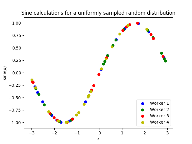
If you want to verify your results through plotting and installed Matplotlib earlier, copy and paste the following code into the bottom of your calling script and run python calling_script.py again

import matplotlib.pyplot as plt

colors = ["b", "g", "r", "y", "m", "c", "k", "w"]

for i in range(1, nworkers + 1):
    worker_xy = np.extract(H["sim_worker"] == i, H)
    x = [entry.tolist()[0] for entry in worker_xy["x"]]
    y = [entry for entry in worker_xy["y"]]
    plt.scatter(x, y, label="Worker {}".format(i), c=colors[i - 1])

plt.title("Sine calculations for a uniformly sampled random distribution")
plt.xlabel("x")
plt.ylabel("sine(x)")
plt.legend(loc="lower right")
plt.savefig("tutorial_sines.png")

Each of these example files can be found in the repository in examples/tutorials/simple_sine.

Exercise

Write a Calling Script with the following specifications:

Set the generator function’s lower and upper bounds to -6 and 6, respectively
Increase the generator batch size to 10
Set libEnsemble to stop execution after 160 generations using the gen_max option
Print an error message if any errors occurred while libEnsemble was running

5. Next steps

libEnsemble with MPI

MPI is a standard interface for parallel computing, implemented in libraries such as MPICH and used at extreme scales. MPI potentially allows libEnsemble’s processes to be distributed over multiple nodes and works in some circumstances where Python’s multiprocessing does not. In this section, we’ll explore modifying the above code to use MPI instead of multiprocessing.

We recommend the MPI distribution MPICH for this tutorial, which can be found for a variety of systems here. You also need mpi4py, which can be installed with pip install mpi4py. If you’d like to use a specific version or distribution of MPI instead of MPICH, configure mpi4py with that MPI at installation with MPICC=<path/to/MPI_C_compiler> pip install mpi4py If this doesn’t work, try appending --user to the end of the command. See the mpi4py docs for more information.

Verify that MPI has been installed correctly with mpirun --version.

Modifying the script

Only a few changes are necessary to make our code MPI-compatible. Note the following:

libE_specs = LibeSpecs()  # class will autodetect MPI runtime

So that only one process executes the graphing and printing portion of our code, modify the bottom of the calling script like this:

...
ensemble = Ensemble(libE_specs, sim_specs, gen_specs, exit_criteria)
ensemble.add_random_streams()
ensemble.run()

if ensemble.is_manager:  # only True on rank 0
    H = ensemble.H
    print([i for i in H.dtype.fields])
    print(H)

    import matplotlib.pyplot as plt

    colors = ["b", "g", "r", "y", "m", "c", "k", "w"]

    for i in range(1, nworkers + 1):
        worker_xy = np.extract(H["sim_worker"] == i, H)
        x = [entry.tolist()[0] for entry in worker_xy["x"]]
        y = [entry for entry in worker_xy["y"]]
        plt.scatter(x, y, label="Worker {}".format(i), c=colors[i - 1])

    plt.title("Sine calculations for a uniformly sampled random distribution")
    plt.xlabel("x")
    plt.ylabel("sine(x)")
    plt.legend(loc="lower right")
    plt.savefig("tutorial_sines.png")

With these changes in place, our libEnsemble code can be run with MPI by

$ mpirun -n 5 python calling_script.py

where -n 5 tells mpirun to produce five processes, one of which will be the manager process with the libEnsemble manager and the other four will run libEnsemble workers.

This tutorial is only a tiny demonstration of the parallelism capabilities of libEnsemble. libEnsemble has been developed primarily to support research on High-Performance computers, with potentially hundreds of workers performing calculations simultaneously. Please read our platform guides for introductions to using libEnsemble on many such machines.

libEnsemble’s Executors can launch non-Python user applications and simulations across allocated compute resources. Try out this feature with a more-complicated libEnsemble use-case within our Electrostatic Forces tutorial.